Causal Flow Diagramming

The Five Steps of Causal Flow Diagramming

There are five steps for defining and analyzing a problem’s cause-and-effect system:

Step 1: Identify major factors.

Step 2: Identify cause-and-effect relationships.

Step 3: Characterize the relationships as direct or inverse.

Step 4: Diagram the relationships.

Step 5: Analyze the behavior of the relationships as an integrated system.

Let’s take the steps one at a time. First, we identify the major factors—the engines that drive the problem. (Note: We are concerned in causal flow diagramming primarily with dynamic factors, those that expand and contract, rise and fall, etc.) Let’s consider five major factors in a typical large manufacturing business: sales, profits, research and development, marketing of new products, and competitors’ marketing of comparable products. (This is, of course, an oversimplified representation. There are many other factors involved, but I am using these five simply to demonstrate the technique.)

The second step is to identify the cause-and-effect linkages among the factors. To do that we use a two-column “Cause-and-Effect Table” (Figure 7-1). In the left-hand column we list the causal factors, in the right-hand column the affected factors, and we draw an arrow between them.

Sales affect profits. Profits affect R&D capability. R&D capability affects the marketing of new products. Marketing of new products affects competitors’ marketing of comparable new products. The marketing of competitive new products affects sales.

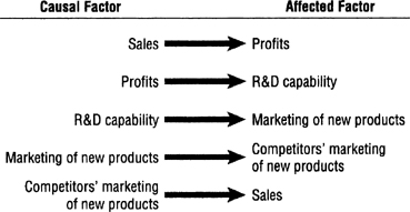
FIGURE 7-1 Cause-and-Effect Table

The third step is to characterize these cause-and-effect relationships as direct or inverse. If the affected factor increases as the causal factor increases and decreases as the causal factor decreases, we have a direct relationship (Figure 7-2).

If, in the opposite case, the affected factor increases as the causal factor decreases and decreases as the causal factor increases, we have an inverse relationship (Figure 7-3).

We indicate a direct relationship with a “D” and an inverse relationship with an “I” (Figure 7-4). If the affected factor is static, i.e., not dynamic, like “death” or “out of business,” we do not assign it an indicator.

In the fourth step we portray these linkages in a causal flow diagram (Figure 7-5). I recommend drawing a circle around each of the factors to highlight them visually, accentuating their distinctiveness.

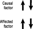
FIGURE 7-2 Direct Relationship

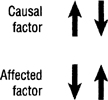
FIGURE 7-3 Inverse Relationship

The most powerful driving force in any cause-and-effect scheme is the so-called feedback loop in which two or more factors are linked circularly in continuous interaction. The behavior of a feedback loop is significant and predictable. If, as in Figure 7-6, all of the linkages are direct relationships, or if there is an even number of inverse linkages, the loop is inherently unstable and will eventually spiral out of control—in either direction. If sales increase, profits increase, R&D increases, marketing of new products increases, causing a further increase in sales, and so on. A “(U)” signifies an unstable feedback loop, a dynamo that drives and powers the cause-and-effect system.

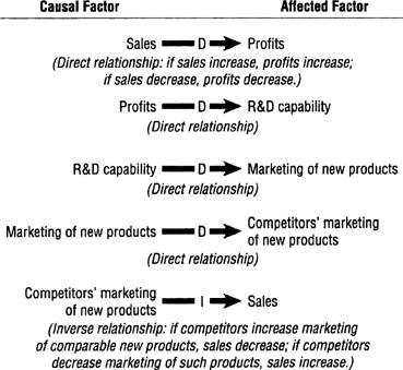
FIGURE 7-4

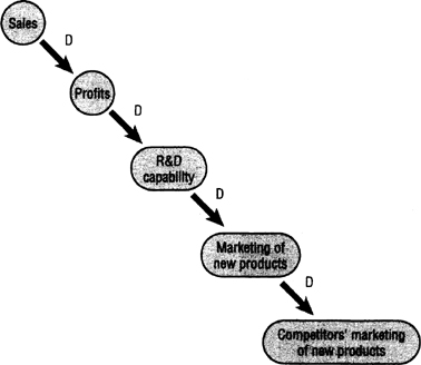
FIGURE 7-5 Causal Flow Diagram

If there is an odd number of inverse linkages, as in Figure 7-7, the loop is inherently self-stabilizing and will achieve equilibrium at some point. If sales increase, profits increase, R&D increases, and marketing of new products increases; but competitors’ marketing of new products also increases, causing sales to decrease. When sales decrease, so do profits, R&D, marketing of new products, and competitors’ marketing of new products, resulting in increased sales. And so the causal flow interactions increase and decrease cyclically. An “(SS)” signifies a self-stabilizing feedback loop, a governor that controls and regulates the cause-and-effect system.

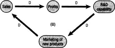
FIGURE 7-6

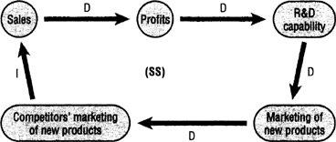
FIGURE 7-7 Self-Stabilizing Feedback Loop

In the fifth and final step we analyze the behavior of the system as an integrated whole, seeking to determine which factors are the most influential. And when a problem occurs, we analyze which factor is creating the problem and how the problem might be resolved by modifying or eliminating factors or introducing new ones.

One way (sort of a sanity check) of validating whether we have accurately portrayed the cause-and-effect relationships is to add a value of +1 to any factor and see how this increment affects the system as a whole. Let’s try this method on Figure 7-7, beginning with “sales.”

If we increase the value of “sales” by 1, the value of “profits” increases by 1 because there is a direct relationship between the two factors (see First Cycle, Figure 7-8). “R&D capability” then also increases by 1, as do “marketing of new products” and “competitors’ marketing of new products.” But then in the Second Cycle the value of “sales” decreases by 1 because of its inverse relationship with “competitors’ marketing of new products.” This decrease starts a new cycle, decreasing the value of each of the other factors by one, which causes the value of “sales” in the Third Cycle to increase by one, triggering yet another cycle. The cycles show how the value of each factor alternates between positive and negative, reflecting the self-stabilizing nature of this feedback loop.

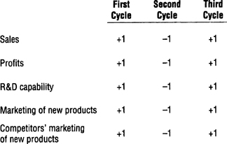
FIGURE 7-8